Quantitative easing by the Fed refers to an unconventional monetary policy tool that made headlines during the 2008 Financial Crisis, and more recently during the Covid-19 pandemic.

What is quantitative easing and why do economists refer to it as unconventional? Why do critics believe that quantitative easing could lead to a rapid rise in inflation rates, and possibly to the worst nightmare of central bankers – stagflation?

Let’s take a deeper look at this monetary policy tool by the Fed and how traders and investors can take advantage by anticipating the next Fed’s QE.

Quantitative Easing Explained

Quantitative easing refers to an unconventional monetary policy in which a central bank, like the Federal Reserve, purchases long-term debt securities on the open market in order to keep interest rates low.

Lower interest rates mean money becomes more accessible for firms and individuals to invest and spend, which in turn should increase economic activity and encourage growth.

That’s why quantitative easing is usually performed during periods of economic distress, such as during recessions and periods of rising unemployment rates.

Understanding the inverse relationship between the price of debt securities, such as bonds, and interest rates is very important to get a grasp of quantitative easing. As bond prices rise, interest rates fall, and vice-versa. And as a central bank keeps buying bonds on the open market, the rising demand leads to higher prices and thus lower interest rates.

Central banks aim to keep interest rates at a level that helps maintain price stability in the market, i.e. most central banks in developed economies aim to achieve an inflation rate of around 2%.

As a country’s economy heats up and prices of goods and services start to rise, central banks hike interest rates to cool down the economy and stabilize inflation. Similarly, when the economy is doing poorly, lower interest rates help support economic activity, which in turn has a positive effect on inflation. One method to lower interest rates is through quantitative easing.

Purpose of Quantitative Easing

Quantitative easing is called an unconventional monetary policy tool because it’s only used when traditional open market operations of a central bank, like the Federal Reserve, for example, lose their effectiveness. This is usually the case when interest rates are either at or approaching zero, which for the most part has been the case since the 2008 Financial Crisis.

Quantitative easing helps to increase the money supply in the economy by purchasing debt securities with newly created bank reserves, which also helps banks maintain and increase their liquidity. While buying securities from its member banks, the Fed gives them cash which in turn can be lent out.

The Fed also controls the minimum reserve requirement for commercial banks: A lower reserve requirement means banks have more cash to lend to companies and individuals, while a higher reserve requirement has the opposite effect. Along with changes in the Fed funds rate, those are the main tools the Fed has at their disposal to support and encourage economic growth, full employment, and price stability.

However, since quantitative easing expands a central bank’s balance sheet, this monetary policy tool itself can also lose effectiveness if used in excess amounts. This is when a country’s fiscal policy comes into play to increase the money supply in the economy as governments can also be involved in purchasing long-term bond securities. In this case, quantitative easing can be both a tool of monetary policy and fiscal policy.

Fed’s Quantitative Easing and Inflation Rates

Even without an economic background, it’s easy to understand that when the supply of something increases, its value usually starts dropping.

The same is the case with money. As the Federal Reserve, or any other central bank, increases the supply of money, its value starts to decrease. This is the reason why some central banks engage in quantitative easing when inflation rates start dropping, as a decrease in the price level of goods and services can also be used as a gauge of the overall economic activity.

However, some economists disagree on whether quantitative easing causes inflation. For example, the Bank of Japan has been repeatedly engaged in quantitative easing since the 1990s, although without much success.

Similarly, when the Federal Reserve started their quantitative easing program in the years following the 2008 Financial Crisis, many economists warned about an upcoming surge in inflation. Still, inflation rates in the United States remained stubbornly low.

Understanding Business Cycles

To understand how the Fed’s quantitative easing works and when the central bank engages in it, it’s mandatory to get a grasp of business cycles and how they affect the economy.

There are four main business cycles: the expansionary phase, the boom or peak phase, the recessionary phase, and the depression or trough phase.

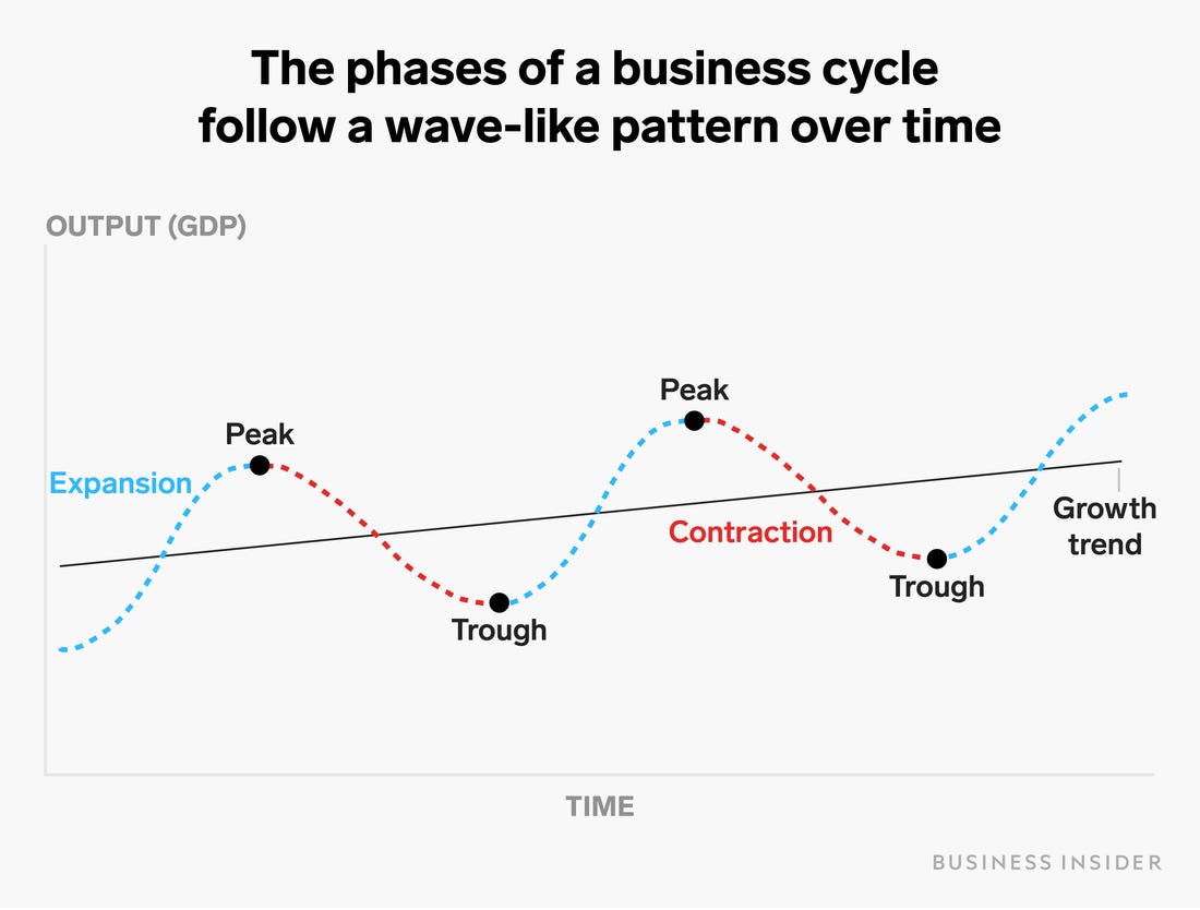
Graphic Source: Business Insider

• Expansion – As its name suggests, economic activity expands during the expansionary phase. This is the spring of the economy. It becomes easier for people to find jobs, money and loans are available, and inflation starts to pick up as individual income grows.

There are two expansionary phases that we need to separate: early expansion, and late expansion. During the early expansionary phase, stocks and commodities are usually starting a new uptrend, bonds are rising in price, and consumer confidence grows.

All these factors lead to inflationary pressures and rising prices of goods and services. As markets are focused on the inflation rate of the United States to anticipate a possible rate hike, the US dollar starts rising as well.

The late expansionary phase is characterized by rising stocks and commodities, but the price of bonds (especially government bonds) is slowly starting to form a top. The reason behind this is again the inverse relationship between bond prices and interest rates.

Since markets are focused on a possible rate hike by the Fed, investors and big players start selling their bond holdings in anticipation of higher interest rates – and therefore falling bond prices.

During the late expansion, inflation rates usually continue to grow.

• Peak – The peak phase of a business cycle starts when the economic activity reaches its top. Jobs are easily available, the economy booms, inflation continues to rise, and signs appear that the economy is about to overheat.

During this phase, stocks and commodities can either continue to rise, reaching record highs, or enter a sideways market. Bond prices continue to fall as markets are convinced that the Federal Reserve has to hike rates in order to cool the economy down. This usually happens when the inflation rate is rapidly approaching the 2% mark.

• Recession – After the economy reached its top, it’s time for the recessionary phase. Stocks and commodities switch from an uptrend to a downtrend, bond prices start to rise because of flight to quality (risk aversion) and the anticipation of interest rate cuts, and the GDP falls.

This is the time when the Federal Reserve could eventually engage in quantitative easing in order to support a fragile economy, job production, and increase inflationary pressures. Every quarter, the FOMC holds a monetary policy meeting where board members assess the current economic activity, after which a press release informs the market about any change in monetary policy and interest rates. Markets always keep an eye on the FOMC meetings which can send shockwaves through the market and heavily impact the value of the US dollar.

• Though – Finally, the though phase (or depression) is characterized by falling or sideways moving stocks and commodities, rising prices of safe havens like US Treasuries, and a falling US dollar. 

This is the time when prudent investors start investing in undervalued stocks since the though is followed by an economic expansion. The Fed can continue with their quantitative easing program during this phase as long as economic activity picks up again.

Yield Curve and Business Cycle

Yield curves are closely connected to the current phase of the business cycle, which makes them an important topic to explore when talking about the Fed Reserve quantitative easing. A yield curve is simply a line that connects the yields, or interest rates, of bonds that have different maturity dates.

For example, a trader or investor could take the 6-month, 2-years, 5-years, 10-years, and 30-years US Treasuries to draw a yield curve, where the x-axis refers to the maturity of the bond, and the y-axis to the yield of the bond.

Market participants are very focused on the current state and changes in the yield curve as it provides valuable clues about the current state of the economy, as well as future changes in interest rates. When talking about interest rates, it’s important to note that bullish on interest rates means a falling interest rate, and bearish on interest rates means a rising interest rate.

It’s also crucial to understand that short-term bonds, like the 2-year Treasury, usually reflect expectations of future Fed interest rates, while long-term bonds, like the 10-year and 30-year Treasuries, reflect future inflation rate expectations.

Now, it’s time to introduce various combinations of yield curves that can help predict a Fed’s QE. Here’s an overview of the main yield curve environments.

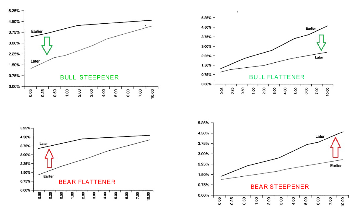
• Bull Flattener – A bull flattener is an environment in which rates on long-term Treasures are falling more quickly than rates on short-term Treasuries. Here, bullish means falling long-term yields, and “flattener” means the yield curve is becoming flatter than before. 

A bull flattener usually occurs during the recessionary phase when stocks, commodities, the US dollar, and the GDP are falling, while bonds and safe havens are entering into a fresh uptrend. During this phase, markets decrease their future inflation rate expectations, which leads to lower yields on the long end of the yield curve.

There are also no expectations of a rate hike by the Fed, which leaves rates on the short end unchanged. Bull flatteners are often used to anticipate an upcoming monetary easing by the Fed.

• Bear Flattener – A bear flattener is an environment in which rates on the short end are rising more quickly than rates on the long end of the yield curve. Here, bear means that short-term interest rates are rising, while “flattener” again means that the yield curve is overall becoming flatter than before.

Bear flatteners usually occur during the early recessionary phase, when both stocks and bonds enter a downtrend. They are also an early sign of an upcoming quantitative easing cycle.

• Bull Steepener – During a bull steepener, interest rates on short-term Treasuries are falling quicker than rates on long-term Treasuries. Bull steepeners usually occur after the economy hits the bottom during the depression phase, and when most asset classes slowly start to recover lost ground in the coming weeks and months.

Since the economy is still fragile and needs support from the central bank, bull steepeners often form after the Fed engages in quantitative easing or applies another accommodative monetary policy tool.

• Bear Steepener – Finally, a bear steepener usually occurs during the late expansionary phase when almost all asset classes rise in value, as well as inflationary pressures. In a bear steepener, yields on long-term Treasuries rise more quickly than yields on short-term Treasuries, reflecting investor expectations about rising inflation rates. A bear steepener is usually followed by monetary tightening by the Fed during the peak phase.

How to Anticipate a Fed Quantitative Easing Cycle?

So far, we’ve covered what the Fed quantitative easing is and how it is used to support economic growth, the labor market, and price stability. You’ve also learned how business cycles and yield curves are connected with quantitative easing and in which phases this monetary easing usually occurs.

The best way to anticipate a Fed quantitative easing cycle is to observe the economy and subtle signs that provide hints about the current economic activity. Following the current business cycle and yield curves are one way to do so.

The Federal Reserve QE program usually takes place after the trough phase, when economic activity hits rock bottom. Most asset classes are falling except safe havens, and the US dollar starts slowly to recover from heavy selling pressure. This is the period when the Fed may decide to further support the economy by purchasing Treasuries from their member banks and increasing the money supply.

Regarding the yield curve, the US Fed quantitative easing usually begins when the yield curve forms a bull flattener, which is the late recessionary phase and continues through the trough phase.

Besides the business cycle and the yield curve, market reports are also a powerful tool to forecast an upcoming US Fed quantitative easing. Look out for strong changes in leading economic indicators, such as new housing starts, consumer confidence, and Purchasing Manager Indices (PMIs). When leading indicators become weak, there is a high chance that the Fed will engage in quantitative easing.

Fed QE Program: Yield Differentials

Let’s take a look at the Fred database to compare the Fed funds rate and the 10-year and 2-year yield differential. The Fed funds rate is the most important interest rate in the market as all other interest rates are derived from it. The 10-year and 2-year yield differential is simply a sign of whether the difference between the long end and short end of the yield curve is expanding or not. An unchanged 10-year yield vs a falling 2-year yield signals a bull steepener, which occurs during periods of quantitative easing.

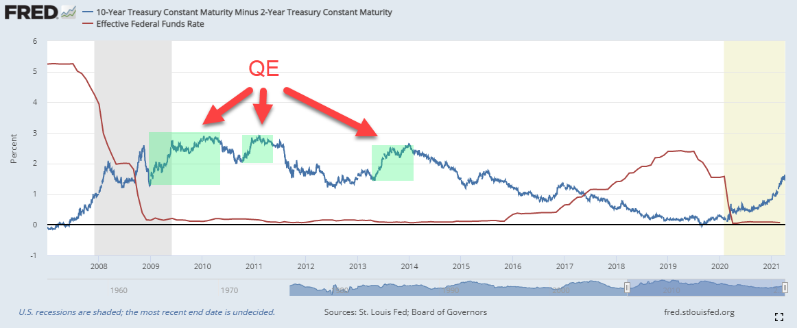
During the QE phases, marked by the green rectangles on the chart, the Federal Reserve purchased short-term government bonds, which in turn pushed their price higher. Due to the inverse price-yield relationship, yields on the short end of the yield curve fell, forming a bull steepener.

Note that QE Fed began when the Federal Funds rate (red line) reached record lows, which made it impossible to further lower interest rates (except to go negative.)

Final Words

According to the textbook quantitative easing definition, a central bank purchases government bonds from banks, thereby pumping cash into the market, which in turn should encourage lending and spending and support economic activity. When demand for bonds rises, their yields fall due to the inverse relationship between bond prices and interest rates. As a result, lower interest rates and accessible money should support economic growth, employment, and price stability.

Quantitative easing is a controversial topic as it doesn’t always return the results expected by economic theory. Japan has been engaged in QE since the early 90s, yet inflation rates remain stubbornly low despite waves of money hitting the economy. QE returns the best results if there are no other monetary and fiscal easing tools available to a country, such as lowering overnight interest rates and minimum reserve requirements.

Still, by anticipating a new cycle of quantitative easing, market participants can position themselves into the right asset classes and take advantage of the lower interest rates. And once the Fed ends QE, a new business cycle begins which can again provide profitable investment opportunities to traders and investors.